
Propensity Scores
Many quasi-experimental analyses will utilize propensity score matching to estimate the average treatment effect (ATE) of an intervention on a sample population. Doing this accounts for relevant confounding factors by the included covariates. A first step in this process is to create a diagram that describes the overall causal model. The diagram below is an example of how variables can be laid out, and how they influence the overall causal model.
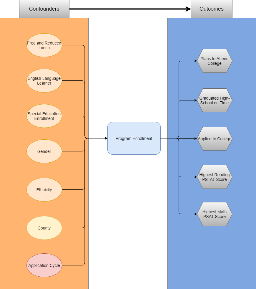
Causal Model
The causal model above describes the relevant covariates that influence either the outcome (enrollment in the program), or the target outcomes of the program.
Propensity Scores
A propensity score can be thought of as the probability that an individual is assigned to a treatment condition. A researcher can utilize a propensity score to approximate causal effects, with reservations, from a data that where participants were not randomly assigned to treatment or control conditions. It can be described in the following equation:
\[ e(W) = P(T=1|W) \]
Where \(T=1\) is the treatment condition, and \(W\) is a set of relevant covariates. Therefore, the calculated value (\(e(W)\)) is the probability (or propensity) that an individual received treatment, given a set of covariates. A benefit of propensity scores, is that even if there are many relevant covariates (high dimensionaltiy of \(W\) ), the result is still a single propensity score (\(e(W)\)).
Conceptually, a researcher can leverage propensity scores to compare treated individuals to control individuals, who look alike based upon the set of relevant covariates (\(W\)), or weight the outcome(s) of interest. This allows the researcher to develop a relevant counterfactual observation to compare to the treated observation, or adjust the outcome(s) accordingly.
Types of Treatment Effects
The Average Treatment Effect (ATE) captures the treatment effect as if the sample population was randomly assigned to treatment or control groups. This is used when participation in the treatment condition is voluntary, and expected to influence only those in the treatment condition.
The average treatment effect on the treated (ATT, ATET, TOT) captures the treatment effect as if the treated population were randomly assigned to treatment or control groups. This is used when you expect all to participate in the target population.
Matching Methods
There are several ways to utilize the calculated propensity (such as matching on the propensity score, or weighting the outcome). The results of these methods should be similar, as long as the researcher has captured all relevant variables that influence the probability of treatment, and the target outcome(s).
Nearest Neighbor
The nearest neighbor method utilizes the propensity score, which summarizes the demographic / psychographic information of the subject into a single metric, to compare observations in different groups. The benefit, is that as the covariates increase in number (thus increasing in complexity) the propensity score remains as a single value.
When leveraging propensity scores in a matching method, it is important to examine the distribution of the propensity scores themselves between the treated and control groups. The overlap of the distributions (those scores that fall within the same range) define the sample that can be utilized for analyses (the global minimum, and maximum, of the two distributions). The researcher must also decide the caliper (or distance between scores) that qualify a “match” between the two groups.
A method to provide evidence that a good caliper has been utilized, is to compare means of the relevant covariates that were used to calculate the propensity score between the treated and control groups of the new “matched” subjects. The standardized mean differences should be in an acceptable range between the two groups.
Inverse Propensity Weighting
A popular use case of propensity scores is to leverage them in a weighting adjustment when estimating the effects of a treatment condition on an outcome. The weighting adjustment has a main benefit over the matching methods described above, specifically that it does not remove units without a relevant match between the two groups.
The use of the propensity score differs depending upon whether the researcher wishes to estimate the average treatment effect (ATE), or the average treatment effect for the treated (ATT).
Estimates for the average treatment effect (ATE), are calculated by leveraging the propensity score for both the treatment and control groups. For the treatment group, the propensity (\(w\)), is calculated as \(w=\frac{1}{p}\). For the control group, the propensity is calculated as \(w=\frac{1}{1-p}\). The result is that treatment subjects who have a high propensity to be treated, are not heavily weighted. Also, control subjects who had a low propensity to be treated are not heavily weighted. However, treated subjects who had a low propensity for treatment are weighted higher, as are control subjects who had a high propensity for treatment. The table below displays how the propensity (\(p\)), influences the treated and control subjects:
Estimates for the average treatment effect for the treated are calculated by leveraging the propensity for only the control group. For the treatment group, the propensity (\(w\)) is 1. For the control group, the propensity is calculated as \(w=\frac{p}{1-p}\). The result is that the treatment subjects are unchanged (as their are weighted by 1), while control subjects with a high propensity for treatment are weighted higher, and control subjects with a low propensity for treatment are weighted lower. The table below displays how the propensity (\(p\)), influences the control subjects:
Model Specification
Whether the researcher is estimating the ATE or the ATT, they are striving for balance between the covariates. The researcher may need to alter their model specification in order to achieve a proper balance (squared, cubic, interaction terms, etc.). Furthermore, the researcher must examine the range of weights that are being applied. If an individual has an exceptionally low propensity, then their weighting may become astronomically high. Extremely high weights can be recoded and brought into a more reasonable range.
